Your first few hundred tokens come back fast. By token 8,000 the same model on the same GPU is noticeably slower, and the bill is climbing in a way that doesn't feel linear with the work. Nothing about the model changed. What changed is a data structure that's been quietly growing in GPU memory the whole time: the KV cache.
The slowdown isn't the model "thinking harder" about a long prompt. It's bytes. Every token you generate forces the GPU to re-read a cache that got bigger with the previous token, and moving those bytes — not doing the math — is what caps your tokens per second.
The work you'd otherwise repeat
Transformers generate text autoregressively: one token at a time, each new token attending to every token before it. Attention needs a Key (K) and Value (V) vector for each previous position.
Computed naively, every decode step would re-run the K and V projections for the entire history — token 8,000 would recompute the keys and values for tokens 1 through 7,999, throw them away, then do it again for token 8,001. That's quadratic work for something that never changes: the K and V for token 500 are identical no matter how long the sequence gets.
Enter the cache
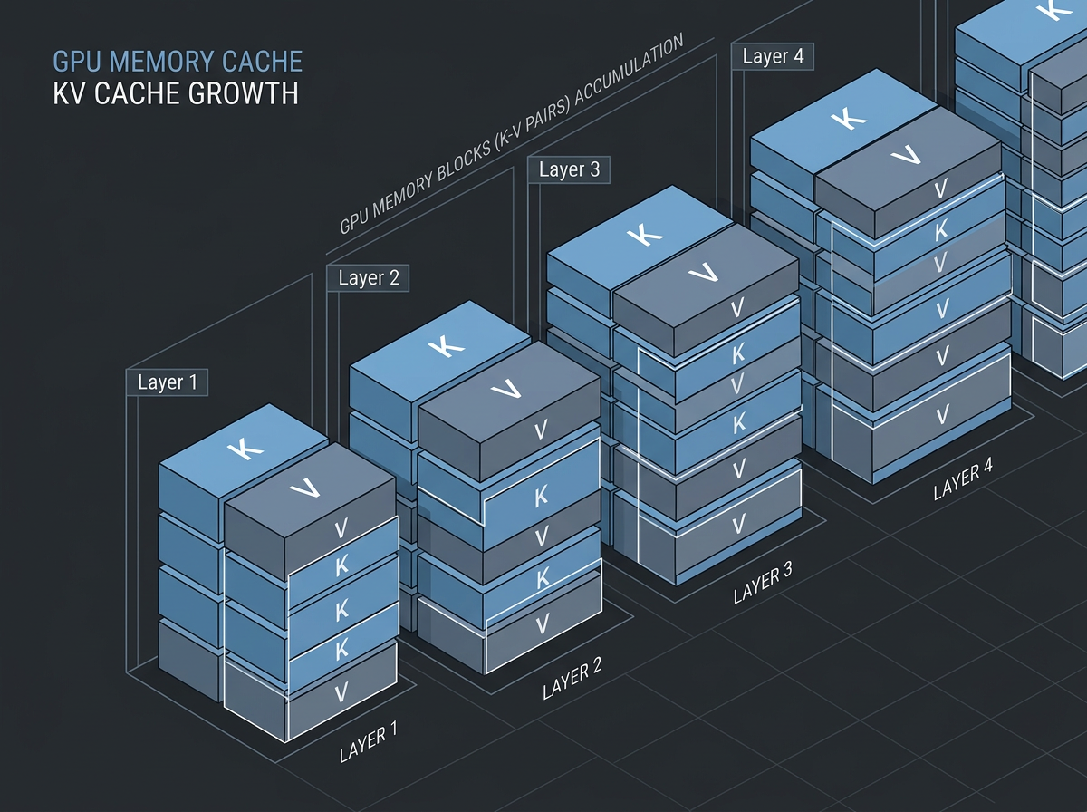
So you keep them. The KV cache stores the K and V vectors for every token already processed, at every layer, for every attention head. A new token computes only its own K and V, appends them, and attends against everything already in the cache.
Per-step attention goes from "recompute over all n tokens" to "compute one, read n." That trade is why generation is practical at all.
The catch is in that word read. You've turned a compute problem into a memory problem, and memory is where it bites.
It grows, term by term
Here's the whole size story in one line:
KV cache bytes = 2 × num_layers × num_kv_heads × head_dim × seq_len × batch_size × bytes_per_element
Walk the terms:
- 2 — you store both K and V.
- num_layers — every transformer layer keeps its own cache.
- num_kv_heads — one entry per KV head; this is the term GQA and MLA attack (more below).
- head_dim — the width of each head's vector.
- seq_len — total tokens in context. This is the one that runs away.
- batch_size — concurrent sequences. The cache is per-request.
- bytes_per_element — 2 for FP16/BF16, 1 for FP8.
Two of these you control at inference time, and both are linear: double the context, double the cache; double the concurrent users, double the cache.
What that costs in practice
Numbers make it real.
| Model | Precision | Context | KV cache |
|---|---|---|---|
| Llama-2-7B | FP16 | per token | ~0.5 MB |
| Llama-2-7B | FP16 | ~28k tokens | ~14 GB |
| Llama 3.1 70B | BF16 | 128K, 1 user | ~42.9 GB |
For Llama-2-7B, ~14 GB of cache is roughly the size of the model's own FP16 weights. For Llama 3.1 70B at full 128K context, a single sequence's cache is ~43 GB — and that's before you serve a second user.
The pattern: for short prompts, weights dominate memory; for long contexts, the cache dominates, and it's what decides whether the workload fits in VRAM and how fast it runs.
What it looks like on one machine
Those figures come from other people's papers and blog posts. Here is the same effect measured on hardware I can actually put my hands on: an Apple M5 with 32 GB of unified memory, Ollama 0.33.3, and llama3.2 — a 3.2B model at Q4_K_M with an f16 KV cache. Each row fills its window with filler text, generates up to 128 tokens, three times, median reported.
num_ctx |
Prefill | Generation | Resident memory | Wall time |
|---|---|---|---|---|
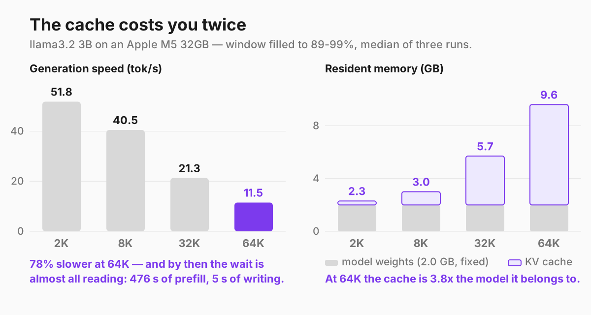
| 2,048 | 1,257 tok/s | 51.8 tok/s | 2.3 GB | 3.1 s |
| 8,192 | 777 tok/s | 40.5 tok/s | 3.0 GB | 12.9 s |
| 32,768 | 275 tok/s | 21.3 tok/s | 5.7 GB | 112.6 s |
| 65,536 | 137 tok/s | 11.5 tok/s | 9.6 GB | 483.8 s |
Read the last column first. The same request — fill the window, write a short answer — takes 3.1 seconds at 2K of context and 484 seconds at 64K. Same model, same machine, a hundred and fifty times the wall clock.
Where that time goes shifts completely along the way. At 2K the request splits about evenly between reading the prompt and writing the answer. At 64K it is 98% reading: 476 seconds of prefill against 5 seconds of generation. Long context does not mainly make the model write slower. It makes it read for eight minutes before it writes anything.
It does write slower too. Generation falls 78%, from 51.8 to 11.5 tok/s, because every new token attends over a cache that is now thirty-two times larger. Prefill falls 89%, because attention over the prompt costs roughly the square of its length.
The memory column is the part that surprised me. This model's weights are 2.0 GB. At 64K the process holds 9.6 GB — the cache has grown to nearly four times the size of the model it belongs to. The thing most people picture as "the model in memory" is the smaller half.
Does the formula hold?
The arithmetic from the last section says 2 × 28 layers × 8 KV heads × 128 × 2 bytes = 112 KiB per token. Against the measured numbers:
num_ctx |
Formula (cache + 2.0 GB weights) | Measured | Gap |
|---|---|---|---|
| 8,192 | 2.88 GB | 3.0 GB | 0.13 |
| 32,768 | 5.50 GB | 5.7 GB | 0.20 |
| 65,536 | 9.00 GB | 9.6 GB | 0.60 |
Close, and wrong in a consistent direction. The formula accounts for about 95% of what the process actually holds, and the gap grows in proportion to context — that residue is the compute buffers, which scale with sequence length too. Use the formula for planning, then add a margin.
What did not happen
At 64K the model was still reported as running entirely on the GPU. Nothing spilled. On a 32 GB machine with a 3B model, the wall you hit is time, not memory — eight minutes of reading before the first word makes the context unusable long before it makes it impossible.
That reverses on bigger models, and the 3.8x ratio above is why: push the weights up and the cache scales right along with them.
The architecture decides whether any of this applies
Everything above assumes every layer attends to every previous token. That is what Llama does, and it is what the formula in this article describes. It is not what every model does.
I ran the same sweep against a Gemma 4 E4B build, which uses sliding-window attention — most of its layers only look back a fixed 512 tokens rather than over the whole sequence. You can read that straight out of the model file: gemma4.attention.sliding_window = 512. Llama 3.2 has no such key.
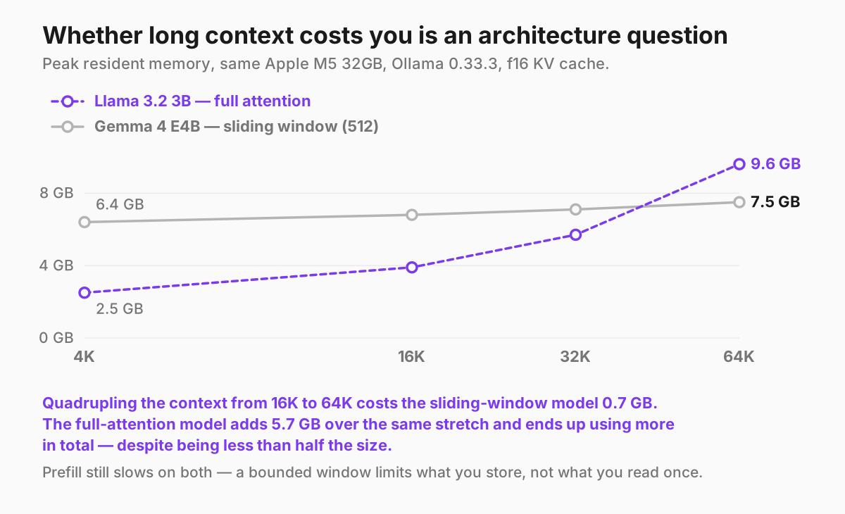
| Context | Llama 3.2 3B (full attention) | Gemma 4 E4B (sliding window) |
|---|---|---|
| 4K | 2.5 GB | 6.4 GB |
| 16K | 3.9 GB | 6.8 GB |
| 32K | 5.7 GB | 7.1 GB |
| 64K | 9.6 GB | 7.5 GB |
Gemma starts far heavier — it is an 8B model against a 3.2B one, and the weights show. Then it stops growing. Quadrupling the context from 16K to 64K costs it 0.7 GB. It costs Llama 5.7 GB, and somewhere around 40K the smaller model overtakes the larger one and never gives the lead back.
Generation tells the same story from the other side. Llama loses 78% between 2K and 64K. Gemma loses 37% between 4K and 64K — 34.5 tok/s down to 21.6 — and by 64K the bigger model is writing at nearly twice the speed of the smaller one, 21.6 against 11.5.
Prefill degrades for both, and steeply: Gemma's falls from 917 to 356 tok/s, Llama's from 1,257 to 137. Sliding windows bound what you have to store, not what you have to read once on the way in.
So before you budget memory from the per-token formula, check whether the model uses sliding-window, grouped-query, or multi-query attention. For a model like Gemma the formula overestimates the cache at long context badly, and the "long context eats your VRAM" warning that motivated this whole article mostly doesn't apply. I took that question further in a four-model comparison on the same machine, where the gap decides which models are usable at 64K and 128K at all.
Measuring it yourself
Four things will silently ruin the numbers, and I hit all four before the table above settled.
num_ctx is fixed when the model loads. Changing it without unloading gets you the previous value. Run ollama stop <model> between measurements or every row comes back identical.
Ollama truncates an over-long prompt to exactly half the window, with no error. I sized the filler text with the usual "English is about 1.33 tokens per word," which is wrong for this model — its real ratio on this filler is 1.57 — so the prompt overshot and came back silently halved: num_ctx / 2 + 2 tokens every time. I was measuring 32K while believing I was measuring 64K. Check prompt_eval_count against num_ctx on every response, and calibrate the ratio by asking the model rather than assuming it.
num_predict is a maximum, not a target. My prompts ended with an instruction to answer in one word, and the model obliged: eval_count came back as 2 or 3. Those first tokens arrive with the cache freshly warm from prefill, so the rate they imply is not the sustained decode rate. Measured on this model at 16K, with only the generation length changing: 3 tokens reads 38.9 tok/s, 14 tokens 29.1, 40 tokens 28.8, 96 tokens 28.7. A 3-token sample reads 35% fast. Generate at least a few dozen tokens and check eval_count every time.
Single runs are noise. My first attempt generated a fixed 64 tokens per context and reported that generation got faster as context grew — 31, then 39, then 36 tok/s. Run-to-run variance on a laptop is around ±25%, which is larger than the effect at small context sizes. Three runs and a median made the trend above appear.
Machine state matters just as much, and I have numbers for that too. I ran the whole sweep twice: once with an image-generation stack holding 17.5 GB of wired memory, and once after it released. Every speed figure in the busy run came back 13–32% low. The memory column, meanwhile, was identical to the decimal — allocation is deterministic, timing is not. The table above is the idle run. If something else on the machine is holding memory, you are measuring that instead.
Why a bigger cache means slower tokens
This is the part the title promises, and it comes down to the two phases of inference behaving completely differently.
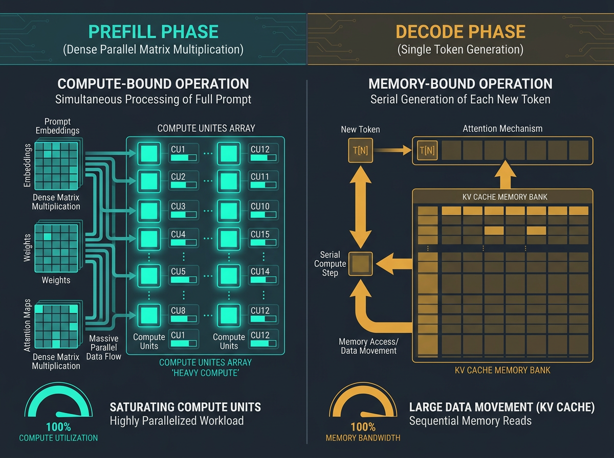
Prefill — processing your prompt — is compute-bound. The whole prompt goes through in parallel as large matrix–matrix multiplications that saturate the GPU's FLOPs. Cost scales roughly quadratically with prompt length, but the hardware is busy doing math, which is what it's good at.
Decode
— generating one token at a time — is memory-bandwidth-bound. Each step does very little math (matrix–vector work for a single new token) but has to stream the model weights and read the entire KV cache out of memory. The GPU isn't limited by how fast it can multiply. It's limited by how fast it can move bytes.
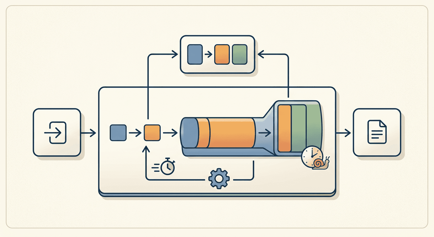
Put those together and the slowdown is mechanical. Every generated token re-reads the whole cache. The cache got bigger when you generated the previous token. More context → more bytes moved per step → fewer tokens per second. The model isn't working harder. It's waiting on memory.
The second tax: concurrency
Bandwidth caps single-stream speed. Capacity caps how many streams you can run at once. The cache shares VRAM with the weights, so every gigabyte of cache is a gigabyte you can't spend on batching more users or allowing longer contexts. That's why a server comfortable with 50 short-prompt users can choke on 10 long-context ones — same model, the cache just ate the headroom.
How people fight the cache
Every serious optimization targets a specific term in that formula, or the bandwidth it implies.
| Technique | What it attacks | Effect |
|---|---|---|
| Grouped-Query Attention (GQA) | num_kv_heads | Query heads share fewer KV heads (e.g. 32 → 8) for a ~4× smaller cache with negligible quality loss. Standard across all Llama 3 sizes. |
| Multi-head Latent Attention (MLA) | num_kv_heads / head_dim | Stores a small latent vector per token and reconstructs K/V on the fly. ~10× smaller cache; used in DeepSeek-V3. |
| PagedAttention (vLLM) | wasted / fragmented memory | Manages the cache in fixed-size blocks like OS paging. Cuts waste from 60–80% down to under 4%, for 2–4× throughput at the same latency. |
| Prefix caching | recompute of shared prefixes | Reuses the KV blocks of an identical prompt prefix across requests. Big win for system-prompt-heavy and agentic workloads. |
| KV quantization / offload | bytes_per_element / location | FP8 or INT4 cache, or spilling to CPU memory — trade precision or bandwidth for capacity. |
GQA and MLA shrink the cache at the architecture level, so you inherit them by picking the right model. PagedAttention and prefix caching are properties of your serving stack — vLLM and SGLang hand them to you. Quantization and offload are the knobs you turn when you're out of VRAM and willing to trade.
The mental model to keep
Context length is a memory-bandwidth tax, and you pay it on every single generated token. That reframes a few decisions. Trimming dead context isn't only about token cost — it directly buys decode speed. Reusing a fixed system-prompt prefix is worth engineering around. And when you pick a serving stack, you're really choosing how well it manages this one cache.
The model's quality lives in the weights; your latency lives in the cache.
References
- Pierre Lienhart — LLM Inference Series: 3. KV caching explained
- Spheron — KV Cache Optimization Guide
- Towards Data Science — Prefill Is Compute-Bound. Decode Is Memory-Bound.
- Kwon et al. — Efficient Memory Management for LLM Serving with PagedAttention (vLLM), arXiv:2309.06180
- DeepSeek-AI — DeepSeek-V3 Technical Report, arXiv:2412.19437
- IBM — What is grouped-query attention (GQA)?